写真は、乱流のスナップショットA Photograph Is a Snapshot of Turbulence
turbulent
photography
二度と同じ配置に戻らない光の、一瞬の実現値。一枚を語る言葉と、統計を語る言葉は違う。A single realisation of light that will never return to the same configuration — and why the language for one frame differs from the language for statistics.
A city intersection never returns to the same configuration.
Stand at the same place, at the same hour, with the same lens, and the arrangement of light and people is different. And yet the character of that intersection survives. The fact that both of these hold at once is the most interesting thing about photography, to me.
It is also exactly the property I have spent years looking at in turbulence.
Turbulence obeys deterministic equations, but small differences in initial conditions separate exponentially, so no individual realisation is reproducible. What is reproducible are the statistics: means, variances, correlations, and spectra.
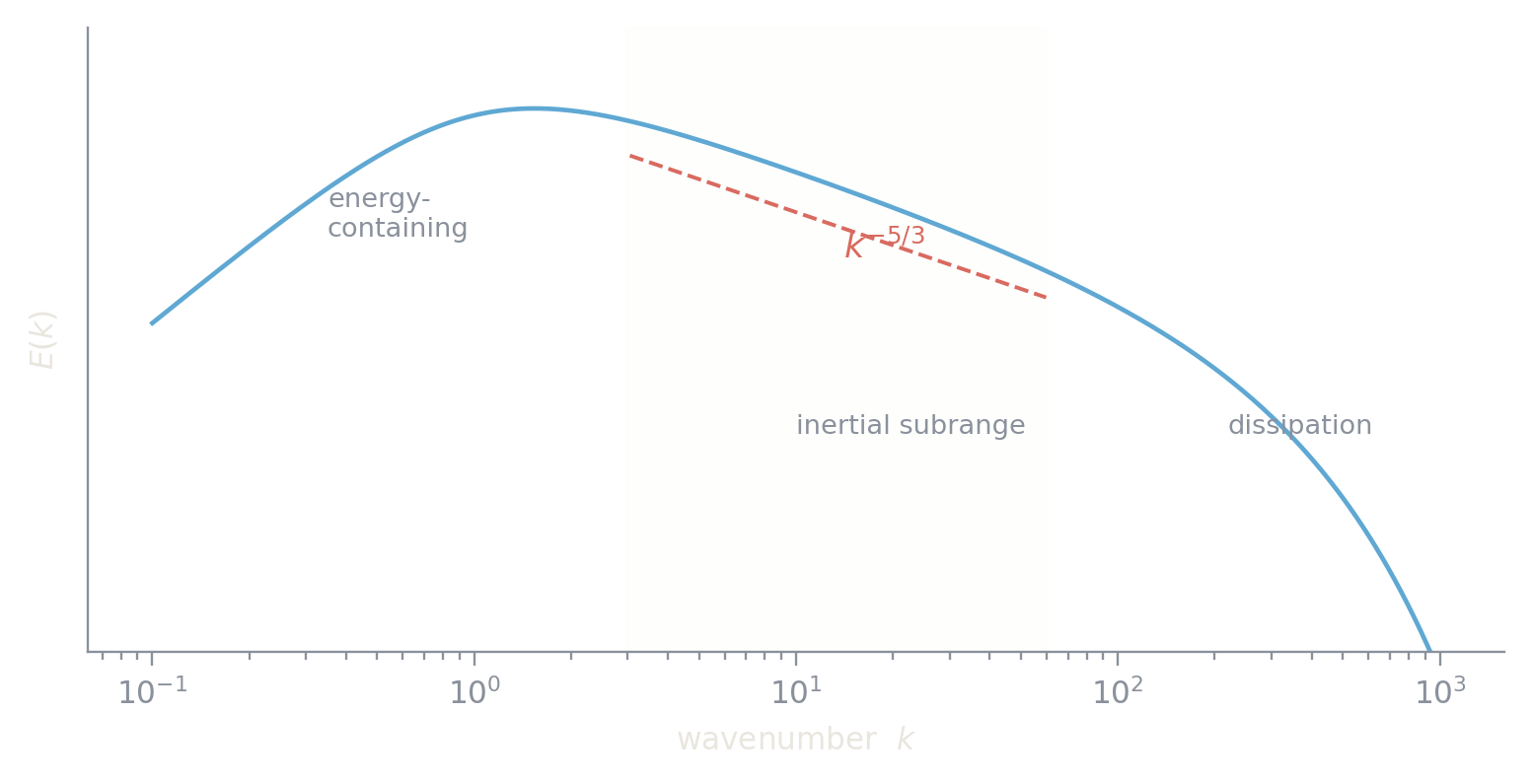
Kolmogorov’s similarity theory states that, in the inertial subrange of a sufficiently high-Reynolds-number flow, the energy spectrum follows
where \varepsilon is the dissipation rate per unit mass, k the wavenumber, and C the Kolmogorov constant. What this describes is not the position of any individual eddy but only how energy is distributed across scales. Nobody can tell you where a given eddy is. The law of the distribution can still be stated.
import numpy as npimport matplotlib.pyplot as pltk = np.logspace(-1, 3, 400)k_L, k_eta =1.0, 200.0# integral and dissipation wavenumbers# von Kármán-type model: -5/3 in the middle, rolled off at both endsE = (k / k_L) **4/ (1+ (k / k_L) **2) ** (17/6) * np.exp(-2.0* k / k_eta)fig, ax = plt.subplots(figsize=(5.6, 2.9))ax.loglog(k, E, color=BLUE, lw=1.2)band = (k >3) & (k <60)ax.loglog(k[band], 0.30* E[band][0] * (k[band] / k[band][0]) ** (-5/3), color=RED, lw=1, ls="--")ax.text(14, 0.30* E[band][0] * (14/ k[band][0]) ** (-5/3) *0.35,r"$k^{-5/3}$", color=RED, fontsize=9)ax.axvspan(3, 60, color=PAPER, alpha=.04)ax.set_xlabel("wavenumber $k$")ax.set_ylabel("$E(k)$")ax.set_ylim(1e-9, 3)ax.set_yticks([])ax.text(0.35, 2e-3, "energy-\ncontaining", color=DIM, fontsize=7)ax.text(10, 2e-6, "inertial subrange", color=DIM, fontsize=7)ax.text(220, 2e-6, "dissipation", color=DIM, fontsize=7, ha="left")fig.tight_layout()plt.show()
Figure 1: A schematic energy spectrum: energy-containing range, the k^(-5/3) inertial subrange, and the dissipative fall-off. Drawn from a model function, not from measurement.
To be explicit: this is a metaphor, not a claim. I am not saying that the luminance field of a photograph obeys Kolmogorov’s law. Natural images are known to have roughly power-law spatial spectra, but that is a separate matter from the turbulent cascade. What is being borrowed here is only the structure of a way of seeing.
Seen this way, it becomes clear that talking about photographs requires two languages.
The language for one frame is a language about an irreproducible realisation: the light of that day, that person’s stride, the way those clouds broke. It vanishes the instant you reduce it to a statistic — which is precisely why single frames are worth making.
The language for a body of work is a language about statistics: what you keep photographing, which scales your eye goes to. It is invisible in one frame and only emerges when a hundred are laid side by side. One’s own “spectrum” turns out to be surprisingly hard to see from the inside.
Not because it can be kept, but because it will never come back.
The turbulent side of this blog will, for a while, move back and forth between those two languages. The DSLR work itself lives in the 藝 section of the hub; how it was made, and what I thought while making it, will live here.