音楽の座標空間 — PODという比喩はどこまで正しいかA Coordinate Space for Music — How Far the POD Analogy Holds
transition
POD
music
楽曲を約8次元の座標に落とす試み。流体で使ってきたモード分解をそのまま持ち込めるのか、どこで壊れるのか。Mapping songs into a ~8-dimensional space. Can the modal decomposition I use for fluids be carried over as-is — and where does it break?
I have come to feel that we search for music almost entirely through tags: chill, for focus, emotional. Every one of them is somebody else’s word, not a coordinate of the sound itself.
In fluids, I fold fields with hundreds of millions of DOF into a few modes. Could the same be done for songs — could music be spanned by around eight axes with physical and perceptual grounding? That is the question at the moment.
同じ演算である / Literally the same operation
まず事実確認から。流体で言う POD と、データ解析で言う PCA は、離散データに対しては同じ演算です。中心化した行列 \mathbf{X} の共分散行列の固有分解、あるいは \mathbf{X} の特異値分解。呼び名が違うのは、適用対象と歴史が違うだけです。
A point of fact first. POD in fluid dynamics and PCA in data analysis are, for discrete data, the same operation: the eigendecomposition of the covariance of a centred matrix \mathbf{X}, or equivalently the SVD of \mathbf{X}. The two names differ only in the field and the history that produced them.
import matplotlib.pyplot as pltfig, ax = plt.subplots(1, 2, figsize=(7.6, 2.7))k = np.arange(1, 13)ax[0].plot(k, np.cumsum(explained[:12]), "o-", color=BLUE, ms=3, lw=1)ax[0].axvline(8, color=DIM, lw=.6, ls=":")ax[0].set_xlabel("number of axes")ax[0].set_ylabel("cumulative variance")ax[0].set_ylim(0, 1.02)P = (np.diag(sig[:2]) @ Vt[:2]).T # songs projected on the first two axesax[1].scatter(P[:, 0], P[:, 1], s=4, color=DIM, alpha=.45, linewidths=0)s =0.9* np.abs(P).max()theta = np.deg2rad(37) # an arbitrary rotation of the same subspacefor (dx, dy), style, c in [((1, 0), "-", BLUE), ((0, 1), "-", BLUE), ((np.cos(theta), np.sin(theta)), "--", RED), ((-np.sin(theta), np.cos(theta)), "--", RED)]: ax[1].plot([-s * dx, s * dx], [-s * dy, s * dy], style, color=c, lw=1)ax[1].set_xticks([]); ax[1].set_yticks([])ax[1].set_aspect("equal")for sp in ax[1].spines.values(): sp.set_visible(False)fig.tight_layout()plt.show()
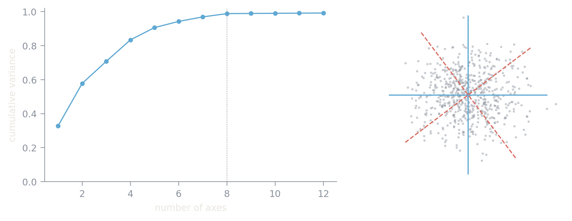
Figure 1: Left: cumulative explained variance — eight axes are enough. Right: the same 2-D cloud with the PCA axes (solid) and an arbitrary rotation of them (dashed). Both reconstruct the data equally well.
1. The axes are fixed by variance, not by meaning. The right-hand figure is the whole argument. Solid lines are the PCA axes; dashed lines are the same axes rotated by 37°. The reconstruction error is identical. The low-dimensional subspace is unique; the choice of axes within it is not. An interpretation such as “axis 3 = brightness” is not something the mathematics hands you — it appears only once you impose extra constraints (sparsity, non-negativity, independence). Eight dimensions are not discovered; they are designed. That is my current conclusion.
2. The features are not linear. A flow snapshot is the physical quantity. A musical “feature” is already a human-made transform. Tempo and loudness are perceived logarithmically, so a linear combination of them need not mean anything.
3. Distance does not match perception. Two songs close in Euclidean distance are not guaranteed to sound alike. In fluids the L^2 norm is tied to energy, a physical quantity; a music coordinate space has no corresponding conserved quantity. Nothing justifies the norm — to me, that is the difference that bites hardest.
I keep going anyway, because the place where an analogy breaks is exactly where a field’s own problem is exposed. That L^2 was the right norm in fluids was good fortune, not a law of nature — a thing I only started to see by working on music.