渦の骨格 — PODは何を捨てているのかThe Skeleton of a Vortex — What POD Throws Away
laminar
POD
turbulence
数億自由度の流れ場を数本のモードに畳む。その圧縮が捨てているものを、合成流れ場のSVDで確かめる。Folding a flow field of hundreds of millions of DOF into a few modes — and checking, on a synthetic field, what that compression discards.
素直であることと、正しいことは違います。この記事は POD の擁護ではなく、POD が何を捨てているかの記録です。
Flow data is large. With 10^7 grid points and 10^3 time steps, a single dataset runs to hundreds of gigabytes. Yet what is actually happening inside it can usually be described by a handful of structures. Proper Orthogonal Decomposition (POD) is the most straightforward tool for pulling those few out.
Straightforward is not the same as correct. This post is not a defence of POD but a record of what POD throws away.
Let u'(\mathbf{x}, t) be the fluctuation left after subtracting the time mean of the velocity (or vorticity) field, and split it into a sum of products of spatial modes \phi_k(\mathbf{x}) and temporal coefficients a_k(t).
In practice one stacks the snapshots as columns of a matrix \mathbf{X} \in \mathbb{R}^{n \times m} (n spatial DOF, m snapshots) and takes its singular value decomposition.
\mathbf{U} の列が空間モード、\sigma_k^2 がそのモードの持つエネルギー、E_r が r 本で再現できるエネルギー比です。POD の最適性は明快で、任意の r 次元線形部分空間の中で、平均二乗誤差を最小にするのは POD 基底であることが示せます。ここに議論の余地はありません。
余地があるのは、「平均二乗誤差が小さいこと」と「流れを理解したこと」が同じか、という点です。
The columns of \mathbf{U} are the spatial modes, \sigma_k^2 is the energy carried by each, and E_r is the fraction of energy recovered by r of them. POD’s optimality is unambiguous: among all r-dimensional linear subspaces, the POD basis minimises the mean-square error. There is no arguing with that.
What is arguable is whether a small mean-square error is the same thing as having understood the flow.
合成場で確かめる / A synthetic check
渦対がゆっくり首を振るだけの、単純な合成渦度場を作ります。物理としては退屈ですが、退屈な流れでこそ POD の癖が見えます。
Here is a synthetic vorticity field: a counter-rotating vortex pair that slowly oscillates. Physically dull — but a dull flow is exactly where POD’s habits become visible.
import numpy as npnx, ny, nt =96, 64, 240x = np.linspace(0, 4* np.pi, nx)y = np.linspace(-2.0, 2.0, ny)X, Y = np.meshgrid(x, y, indexing="ij")t = np.linspace(0, 8* np.pi, nt)def vorticity(tk, sigma=0.35):"""A counter-rotating Gaussian vortex pair, oscillating about x = 2π.""" xc =2* np.pi +1.2* np.sin(0.5* tk) yc =0.6* np.cos(0.5* tk) plus = np.exp(-((X - xc) **2+ (Y - yc) **2) / sigma) minus = np.exp(-((X - xc) **2+ (Y + yc) **2) / sigma)return plus - minus# snapshot matrix: n spatial DOF × m snapshots, time mean removedS = np.stack([vorticity(tk).ravel() for tk in t], axis=1)S -= S.mean(axis=1, keepdims=True)U, sig, Vt = np.linalg.svd(S, full_matrices=False)energy = sig **2/ np.sum(sig **2)cum = np.cumsum(energy)r99 =int(np.searchsorted(cum, 0.99) +1)print(f"snapshot matrix : {S.shape[0]} × {S.shape[1]}")print(f"modes for 99 % : {r99}")
snapshot matrix : 6144 × 240
modes for 99 %  : 5
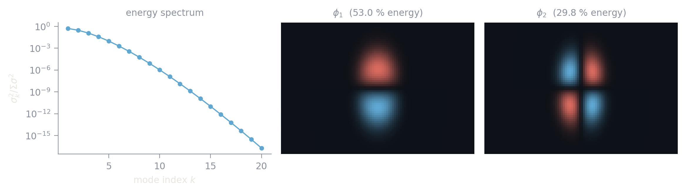
import matplotlib.pyplot as pltfig, ax = plt.subplots(1, 3, figsize=(8.4, 2.4), gridspec_kw={"width_ratios": [1.1, 1, 1]})ax[0].semilogy(np.arange(1, 21), energy[:20], "o-", color=BLUE, ms=3, lw=1)ax[0].set_xlabel("mode index $k$")ax[0].set_ylabel("$\\sigma_k^2 / \\Sigma\\sigma^2$")ax[0].set_title("energy spectrum", color=DIM)lim = np.abs(U[:, :2]).max()for j in (0, 1): ax[j +1].pcolormesh(X, Y, U[:, j].reshape(nx, ny), cmap=VORT, vmin=-lim, vmax=lim, shading="auto") ax[j +1].set_title(f"$\\phi_{j +1}$ ({energy[j] *100:.1f} % energy)", color=DIM) ax[j +1].set_xticks([]); ax[j +1].set_yticks([])for s in ax[j +1].spines.values(): s.set_visible(False)fig.tight_layout()plt.show()
Figure 1: Singular-value spectrum of the synthetic field, and the first two POD modes. Blue is ω < 0, red is ω > 0.
There is exactly one vortex pair, swinging like a pendulum. Even so, recovering 99 % of the energy took 5 modes. The first and second modes are quarter-phase shifted copies of one another — POD has re-expressed a single moving structure as a superposition of several stationary shapes.
捨てているもの / What is discarded
上の実験が示しているのは、POD の三つの性質です。
1. 移流はモードを浪費する。 進行する構造を静止基底で表そうとすると、原理的に sin と cos の対が必要になります。渦が一つしかなくても r は増える。移流が支配的な流れで POD のモード数が膨らむのはこのためで、流れが複雑だからではなく、基底が動かないからです。周波数ごとに分ける SPOD や、単一周波数・単一成長率を持つモードを取り出す DMD が使われるのは、この浪費を避けるためです。
3. 線形部分空間しか張れない。 POD は非線形相互作用そのものを表現しません。表現するのは、非線形相互作用が生んだ「結果」の統計だけです。
The experiment exposes three properties of POD.
1. Advection wastes modes. Representing a travelling structure on a stationary basis requires, in principle, a sine–cosine pair. Even with a single vortex, r grows. That is why mode counts balloon in advection-dominated flows — not because the flow is complex, but because the basis does not move. SPOD, which separates by frequency, and DMD, which extracts modes of a single frequency and growth rate, exist to avoid this waste.
2. The energy ranking is not a ranking of dynamical importance. What \sigma_k^2 orders is variance, not sensitivity. A disturbance that triggers transition can destabilise a system while remaining small in energy. “99 % in the top ten modes” is enough for reconstruction, not necessarily enough for prediction.
3. Only a linear subspace is available. POD does not represent nonlinear interaction itself. It represents only the statistics of what that interaction produced.
Compression is not a decision about what to keep. It is a decision about what may safely be thrown away. Unless the discarded half is written down somewhere, the model begins, quietly, to lie.
次は、同じ道具を音楽に向けたときに何が起きるかを書きます。
Next, what happens when the same tool is pointed at music.